3.2.3 Distribute
The distributive law of real algebra relates the operations of
multiplication and addition; stated symbolically,
 a⋅(b+c)=a⋅b+a⋅c. This can be generalized somewhat to other operators, for example,
 a^(b+c)=a^b⋅a^c.
It can be generalized even further to non-algebraic expressions,
consistent with the dichotomous
operation of
specific and non-specific simplification (§3.2.2).
Informally, algebraic distribution makes expressions
“bigger”. Non-algebraic
distribution also makes expressions bigger.
In this context, Distribute can be thought of as “expansion”.
a^(b+c)=a^b⋅a^c.
It can be generalized even further to non-algebraic expressions,
consistent with the dichotomous
operation of
specific and non-specific simplification (§3.2.2).
Informally, algebraic distribution makes expressions
“bigger”. Non-algebraic
distribution also makes expressions bigger.
In this context, Distribute can be thought of as “expansion”.
3.2.3.1 Algebraic distribution
For algebraic expressions, Distribute applies transformations based on the distributive law.
The
multiplication
operator in an expression
like
 (a+b)⋅(c+d)
can be distributed over the additive operators to yield
(a+b)⋅(c+d)
can be distributed over the additive operators to yield
 a⋅c+a⋅d+b⋅c+b⋅d. Also the
exponentiation
operator in
a⋅c+a⋅d+b⋅c+b⋅d. Also the
exponentiation
operator in
 (a⋅b)^(c⋅d)
can be distributed over the left multiplicative operator to yield
(a⋅b)^(c⋅d)
can be distributed over the left multiplicative operator to yield
 a^(c⋅d)⋅b^(c⋅d).
Applied to
 (a-b)÷c, distribution produces
 a÷c-b÷c
where
c
is any expression.
The transformation is still algebraic because
(a-b)÷c
is
the same as
a÷c-b÷c
where
c
is any expression.
The transformation is still algebraic because
(a-b)÷c
is
the same as
 (a-b)⋅(1÷c). Distributed, this becomes
 a⋅(1÷c)-b⋅(1÷c),
which can simplified to
a÷c-b÷c.
a⋅(1÷c)-b⋅(1÷c),
which can simplified to
a÷c-b÷c.
Distribution can also be used to transform unary operators, for
example
 -(a+b)=-a-b.
The distributive law is slightly different in Boolean algebra.
In particular, the Boolean ∧ and ∨ operators are mutually
distributive. That is, ∧ distributes over ∨ such that  a∧(b∨c) becomes
  a∧b∨a∧c
and ∨ distributes over ∧ so
a∧b∨a∧c
and ∨ distributes over ∧ so  a∨b∧c becomes
  (a∨b)∧(a∨c).
3.2.3.2 Non-algebraic distribution
For non-algebraic applications, Distribute performs an
“expansion”.
It sometimes goes hand-in-hand with simplification, particular when
intermediate transformations
are applied to achieve the simplification. When simplification
performs what would appear to be a drastic reduction, Distribute can be used instead to produce the first intermediate expansion.
A case in point is the binary angle operator applied to two vectors
to produce the cosine of the angle by dividing
the dot product by the square root of the product of the vector lengths.
The intermediate transformation is not obvious when
 (1, 0, 1)ʋ∠(0, 1, 1)ʋ
is simplified to
(1, 0, 1)ʋ∠(0, 1, 1)ʋ
is simplified to
 arccos (1/2)
but expansion shows the dot product and vector lengths clearly as an
intermediate result of
arccos (1/2)
but expansion shows the dot product and vector lengths clearly as an
intermediate result of
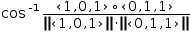 arccos ((1, 0, 1)ʋ∘(0, 1, 1)ʋ÷(|(1, 0, 1)ʋ|⋅|(0, 1, 1)ʋ|)).
The magnitude and dot product operators can be individually expanded to
arccos ((1, 0, 1)ʋ∘(0, 1, 1)ʋ÷(|(1, 0, 1)ʋ|⋅|(0, 1, 1)ʋ|)).
The magnitude and dot product operators can be individually expanded to
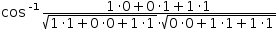 arccos ((1⋅0+0⋅1+1⋅1)÷(√(1⋅1+0⋅0+1⋅1)⋅√(0⋅0+1⋅1+1⋅1))).
Other useful distribution-like transformations are provided.
Special cases exist for logs,
derivatives, integrals, collections and generators.
For example, distribution applied to a generator expands the
generator, provided the domain is constant.
That is
 ((x, x^2)|x∈0, 2)
distributes to
((x, x^2)|x∈0, 2)
distributes to
 ((0, 0^2), (1, 1^2), (2, 2^2)).